Stock Market Analysis

Stock Market Analysis:

In this portfolio project we will be looking at data from the stock market, particularly some technology stocks. We will use pandas to get stock information, visualize different aspects of it, and finally we will look at a few ways of analyzing the risk of a stock, based on its previous performance history. We will also be predicting future stock prices through a Monte Carlo method!

We’ll be answering the following questions along the way:

• What was the change in price of the stock over time?
• What was the daily return of the stock on average?
• What was the moving average of the various stocks?
• What was the correlation between different stocks’ closing prices?
• What was the correlation between different stocks’ daily returns?
• How much value do we put at risk by investing in a particular stock?
• How can we attempt to predict future stock behavior?

Let’s creat a list and call it tech_list

tech_list = ["AAPL","GOOG","MSFT","AMZN","TSLA"]

end = datetime.now()
start = datetime(end.year-1,end.month,end.day)

for stock in tech_list:
    globals()[stock]=pdr.DataReader(stock,"yahoo",start,end)

TSLA

	High	Low	Open	Close	Volume	Adj Close
Date
2019-10-01	49.189999	47.826000	48.299999	48.938000	30813000.0	48.938000
2019-10-02	48.930000	47.886002	48.658001	48.625999	28157000.0	48.625999
2019-10-03	46.896000	44.855999	46.372002	46.605999	75422500.0	46.605999
2019-10-04	46.956001	45.613998	46.321999	46.285999	39975000.0	46.285999
2019-10-07	47.712002	45.709999	45.959999	47.543999	40321000.0	47.543999
...	...	...	...	...	...	...
2020-09-25	408.730011	391.299988	393.470001	407.339996	67208500.0	407.339996
2020-09-28	428.079987	415.549988	424.619995	421.200012	49719600.0	421.200012
2020-09-29	428.500000	411.600006	416.000000	419.070007	50219300.0	419.070007
2020-09-30	433.929993	420.470001	421.320007	429.010010	48145600.0	429.010010
2020-10-01	448.880005	434.420013	440.760010	448.160004	50413600.0	448.160004

254 rows × 6 columns

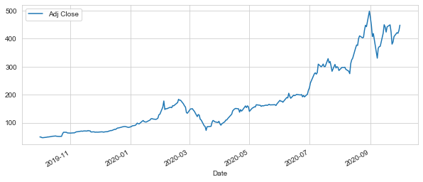
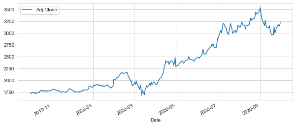
TSLA["Adj Close"].plot(legend=True, figsize=(10,4))

<matplotlib.axes._subplots.AxesSubplot at 0x1ced31a6888>

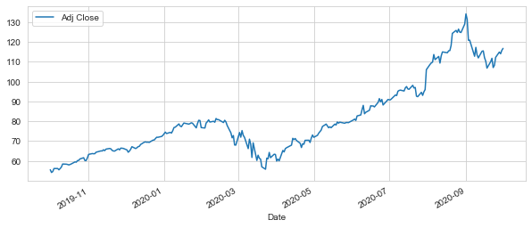
AAPL["Adj Close"].plot(legend=True, figsize=(10,4))

<matplotlib.axes._subplots.AxesSubplot at 0x1ced3168c08>

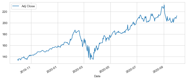
MSFT["Adj Close"].plot(legend=True, figsize=(10,4))

<matplotlib.axes._subplots.AxesSubplot at 0x1ced30c4748>

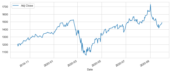
GOOG["Adj Close"].plot(legend=True, figsize=(10,4))

<matplotlib.axes._subplots.AxesSubplot at 0x1ced300d988>

AMZN["Adj Close"].plot(legend=True, figsize=(10,4))

<matplotlib.axes._subplots.AxesSubplot at 0x1ced32efe48>

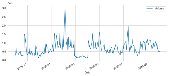
TSLA["Volume"].plot(legend=True, figsize=(10,4))

<matplotlib.axes._subplots.AxesSubplot at 0x1ced3388948>

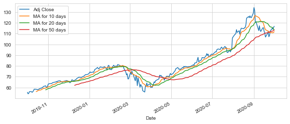
ma_day =[10,20,50]

for ma in ma_day:
    column_name = "MA for %s days" %(str(ma))
    AAPL[column_name]=AAPL["Adj Close"].rolling(ma).mean()

AAPL[["Adj Close","MA for 10 days","MA for 20 days","MA for 50 days"]].plot(subplots=False,figsize=(10,4))

<matplotlib.axes._subplots.AxesSubplot at 0x1ced3647f08>

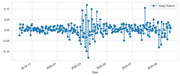
Section 2 - Daily Return Analysis

We’re now going to analyze the risk of the stock. In order to do so we’ll need to take a closer look at the daily changes of the stock, and not just its absolute value. Let’s go ahead and use pandas to retrieve teh daily returns for the Apple stock.

AAPL["Daily Return"] = AAPL["Adj Close"].pct_change()

AAPL["Daily Return"].plot(figsize=(10,4),legend=True,linestyle="--",marker="o")

<matplotlib.axes._subplots.AxesSubplot at 0x1ced397ebc8>

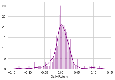
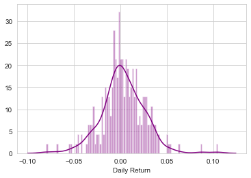
sns.distplot(AAPL['Daily Return'].dropna(),bins=100,color='purple')

<matplotlib.axes._subplots.AxesSubplot at 0x1ced39f01c8>

Now what if we wanted to analyze the returns of all the stocks in our list? Let’s go ahead and build a DataFrame with all the [‘Close’] columns for each of the stocks dataframes.

closing_df=pdr.DataReader(tech_list,"yahoo",start,end)["Adj Close"]

closing_df

Symbols	AAPL	GOOG	MSFT	AMZN	TSLA
Date
2019-10-01	55.595886	1205.099976	135.527100	1735.650024	48.938000
2019-10-02	54.202213	1176.630005	133.134323	1713.229980	48.625999
2019-10-03	54.662643	1187.829956	134.745972	1724.420044	46.605999
2019-10-04	56.194942	1209.000000	136.565262	1739.650024	46.285999
2019-10-07	56.207317	1207.680054	135.576523	1732.660034	47.543999
...	...	...	...	...	...
2020-09-25	112.279999	1444.959961	207.820007	3095.129883	407.339996
2020-09-28	114.959999	1464.520020	209.440002	3174.050049	421.200012
2020-09-29	114.089996	1469.329956	207.259995	3144.879883	419.070007
2020-09-30	115.809998	1469.599976	210.330002	3148.729980	429.010010
2020-10-01	116.790001	1490.089966	212.460007	3221.260010	448.160004

254 rows × 5 columns

Now that we have all the closing prices, let’s go ahead and get the daily return for all the stocks, like we did for the Apple stock.

tech_rets=closing_df.pct_change()

tech_rets

Symbols	AAPL	GOOG	MSFT	AMZN	TSLA
Date
2019-10-01	NaN	NaN	NaN	NaN	NaN
2019-10-02	-0.025068	-0.023625	-0.017655	-0.012917	-0.006375
2019-10-03	0.008495	0.009519	0.012105	0.006532	-0.041542
2019-10-04	0.028032	0.017822	0.013502	0.008832	-0.006866
2019-10-07	0.000220	-0.001092	-0.007240	-0.004018	0.027179
...	...	...	...	...	...
2020-09-25	0.037516	0.011671	0.022787	0.024949	0.050414
2020-09-28	0.023869	0.013537	0.007795	0.025498	0.034026
2020-09-29	-0.007568	0.003284	-0.010409	-0.009190	-0.005057
2020-09-30	0.015076	0.000184	0.014812	0.001224	0.023719
2020-10-01	0.008462	0.013943	0.010127	0.023035	0.044638

254 rows × 5 columns

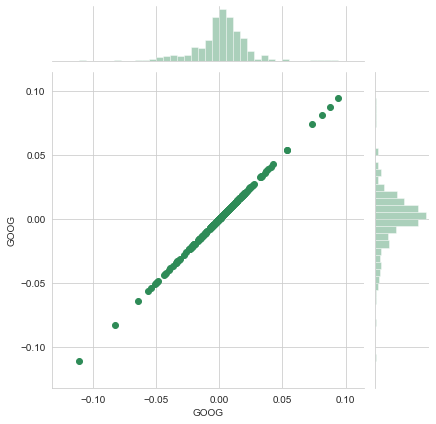
sns.jointplot("GOOG","GOOG",tech_rets, kind="scatter",color="seagreen")

<seaborn.axisgrid.JointGrid at 0x1ced4cf8448>

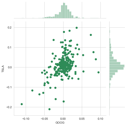
sns.jointplot("GOOG","TSLA",tech_rets, kind="scatter",color="seagreen")

<seaborn.axisgrid.JointGrid at 0x1ced5083d48>

sns.pairplot(tech_rets.dropna())

<seaborn.axisgrid.PairGrid at 0x1ced5e57a88>

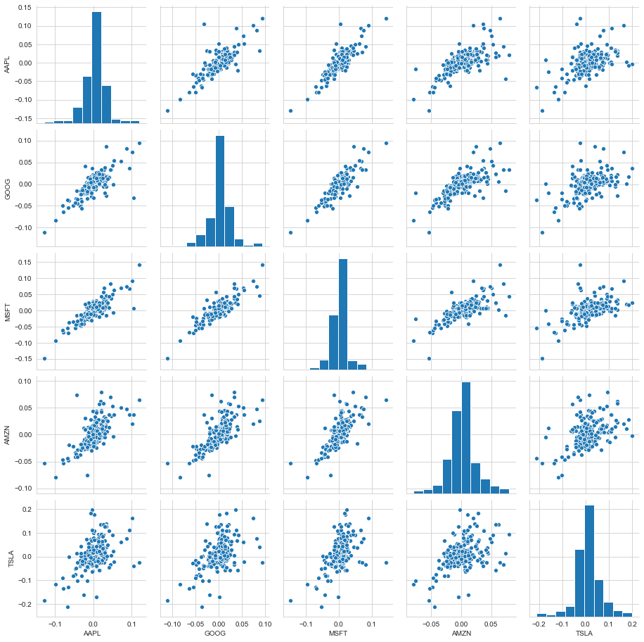
Above we can see all the relationships on daily returns between all the stocks. A quick glance shows an interesting correlation between Google and Amazon daily returns. It might be interesting to investigate that individual comaprison. While the simplicity of just calling sns.pairplot() is fantastic we can also use sns.PairGrid() for full control of the figure, including what kind of plots go in the diagonal, the upper triangle, and the lower triangle.

Section 3 - Risk Analysis

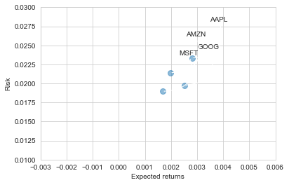
There are many ways we can quantify risk, one of the most basic ways using the information we’ve gathered on daily percentage returns is by comparing the expected return with the standard deviation of the daily returns.

#Let's start by defining a new DataFrame as a clenaed version of the oriignal tech_rets DataFrame
rets = tech_rets.dropna()

area = np.pi*20

plt.scatter(rets.mean(), rets.std(),alpha = 0.5,s =area)

#Set the x and y limits of the plot (optional, remove this if you don't see anything in your plot)
plt.ylim([0.01,0.025])
plt.xlim([-0.003,0.004])

#Set the plot axis titles
plt.xlabel('Expected returns')
plt.ylabel('Risk')

#Label the scatter plots
for label, x, y in zip(rets.columns, rets.mean(), rets.std()):
    plt.annotate(
        label, 
        xy = (x, y), xytext = (50, 50),
        textcoords = 'offset points', ha = 'right', va = 'bottom',
        arrowprops = dict(arrowstyle = '-', connectionstyle = 'arc3,rad=-0.3'))

Value at Risk

Let’s go ahead and define a value at risk parameter for our stocks. We can treat value at risk as the amount of money we could expect to lose (aka putting at risk) for a given confidence interval. Theres several methods we can use for estimating a value at risk. Let’s go ahead and see some of them in action.

Value at risk using the “bootstrap” method

For this method we will calculate the empirical quantiles from a histogram of daily returns. For more information on quantiles, check out this link: http://en.wikipedia.org/wiki/Quantile

# Note the use of dropna() here, otherwise the NaN values can't be read by seaborn
sns.distplot(AAPL['Daily Return'].dropna(),bins=100,color='purple')

Now we can use quantile to get the risk value for the stock.

# The 0.05 empirical quantile of daily returns
rets['AAPL'].quantile(0.05)

-0.03377112705414851

The 0.05 empirical quantile of daily returns is at -0.033. That means that with 95% confidence, our worst daily loss will not exceed 3%. If we have a 1 million dollar investment, our one-day 5% VaR is 0.03 * 1,000,000 = $30,000.